
This week’s article in The Star looked at the effect that the draft lottery has had on the incentive for a team to intentionally try to be bad in order to get the top pick in the draft.
The draft was instituted in 1963 as a way of sorting out how to bring amateur players not currently in the league to NHL teams. This was an era before free agency, meaning that teams owned the rights to players in the league essentially in perpetuity (although these rights could be traded), which had the effect of seriously suppressing salaries. By having a draft (which was an innovation developed by the NFL in 1936), the teams could assign the rights to players outside the league without getting into bidding wars.
It is worth mentioning that the league did in fact have some means in place of assigning the rights to these players. Each team kept a “negotiation list” of young players, and other teams were prevented from dealing with these players. Bobby Hull was infamously put on Chicago’s negotiation list at age 11. However, these negotiation lists were limited in the number of players that a team could have, and so a draft was deemed necessary to assign the rights to the rest of the players. Indeed, for the first several years of the draft, many top picks never even made it to the NHL, and those that did were often not star players. For this reason, in the statistical analysis below, I considered data starting in 1980, when the “NHL Amateur Draft” was renamed to the “NHL Entry Draft”, and became the only way for players under 20 to get into the league (with few exceptions).
The next step, then, was to determine the order in which teams would pick. The NHL again followed the NFL’s lead and went with a reverse order draft in which the worst teams that year would pick first. By doing this, the league would promote parity, which is good for the overall health of the league.
The problem with a reverse order draft, however, is that it can create perverse incentives. Instead of trying to win games, teams might now have an incentive to lose them in order to get a good draft pick, which could make them better off in the long run. This is naturally something that the league would be concerned about, as fans presumably are not as interested in watching a game in which one team is not actually trying to win.
So, in 1995, the NHL adopted a draft lottery, which had first been employed by the NBA in 1985. Starting in 1995, all 14 non-playoff teams would be entered into a lottery in which the probability of winning was greater for teams lower in the standings. However, the winner of the lottery could only move up 4 spaces, meaning that only the bottom 5 teams had a chance to pick 1st overall. This was changed for the 2013 draft, when the limit on how many places a team could move up was eliminated.
The idea behind the draft lottery is that the benefits to being bad (a high draft pick) would be reduced, while leaving the costs the same (reduced attendance and other sorts of revenue), but still there would be an overall improvement in league parity as worse teams would be getting (on average) better players.
So, given this history, the question at hand was to determine what effect (if any) the draft lottery has had on teams’ incentives to tank for a high draft pick.
The first issue that must be addressed in order to answer this question is how to measure the effect? There are many indicators of the incentive to tank, but in this case I decided to keep it simple and look at the points of the last place team. As mentioned in the article, this is not as simple as looking at how last place teams performed before the lottery and comparing that to how they performed after. Accounting for differences in games played is simple enough, but the fact that expansion teams are generally terrible (and expansion for the most part occurred before the introduction of the lottery), and a salary cap was introduced in 2005 and the extra “loser point” in 1999, makes thing more complicated.
The Bettman point has had the effect of increasing the total amount of points allocated in a season, which means that last place teams accumulate more points even if they aren’t any better. This is essentially points inflation. Dealing with inflation is relatively simple. When economists deal with inflation in money, it’s accounted for by considering how much money is required to buy a standard bundle of goods. If that bundle costs $100 in one year and $110 the next, then there has been 10% inflation.
For points, I considered how many points are needed to be average. Before the Bettman point, a point per game (82 points) was average. After the Bettman point, the average increased to 86-87 points in a given 82 game season, and then increased again to 91-92 points after the introduction of the salary cap. The following table shows what the average number of points was each season:
| Year | Average Number of Points |
| 2000 | 86.07143 |
| 2001 | 86.06667 |
| 2002 | 86.03333 |
| 2003 | 87.16667 |
| 2004 | 86.83333 |
| 2006 | 91.3667 |
| 2007 | 91.3667 |
| 2008 | 91.0667 |
| 2009 | 91.4 |
| 2010 | 92.03333 |
| 2011 | 91.9 |
| 2012 | 92 |
| 2013 | 53.4 |
| 2014 | 92.23333 |
Thus, the variable of interest is the number of points the last place team amassed in a given season divided by the average number of points across teams that year. Before the Bettman point, this is exactly equal to points per game, and after the Bettman point, it is a points per game expressed in pre-1999 points, so to speak (just as money measures are often expressed in 1999 dollars, for example). So, in the 2010-11 season Edmonton finished last with 62 points in 82 games, for 0.756 points per game. However, the league average number of points was 91.9, so I considered Edmonton has having earned 62/91.9 = 0.675 points per game (in pre-1999 points).
With regards to the draft lottery, its introduction is a discrete event. There are years (pre-1995) where it was not in effect, and years (1995 and after) where it was (and still is). The way to account for discrete events is through a dummy variable. Dummy variables take a value of 1 when something is true (in this case, when the lottery is in effect) and zero when it is not. Note that the lottery did change in 2013, but there are only two observations on the new system. For the moment, I just considered whether there was a lottery or not, but it would be worth examining the effect of the new lottery when more data are available. The salary cap (and floor) is also a discrete event, and so a dummy variable was used for its presence.
Finally, there are the expansion teams to account for. Given that teams are expected to be bad earlier in their existence, one might consider using the age of the franchise as a variable. However, the effect of being new does decay relatively quickly, and there really isn’t an advantage to being a particularly old franchise (ask Leafs fans), so using age isn’t appropriate. Again, the solution is to use a dummy variable. Here, however, there are more options. One could use a dummy variable for franchises in their first year, another dummy variable for franchises in their second year, and so on. However, there are only so many opportunities for the last place team to be in their first year of existence, so I opted to create dummy variables for the first 3 years of a franchise’s existence and the second 3 years (years 4 to 6).
Given all this, the linear regression model that was considered is:
Pts % = α + β1Lottery + β2SalaryCap + β3Expansion1-3 + β4Expansion4-6
where Pts % represented the last place team’s points percentage accounting for the inflation of the Bettman point, and Lottery, SalaryCap, Expansion1-3, and Expansion4-6 are dummy variables for the respective events. As mentioned above, the data comprises all seasons from 1979-80 to 2013-14, which yields 15 years with no lottery, no extra point, and no salary cap (but considerable expansion), 5 years with the lottery, but no Bettman point or salary cap (and some expansion), 5 years with the lottery, the Bettman point, but no salary cap (and some expansion), and 9 years with the lottery, the Bettman point, and the salary cap (and no expansion).
The results of the regression are given below:
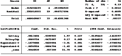
First off, it is worth noting that the R-squared, which is a measure of how well these factors explain the data is 0.4605. This is quite high for anything hockey-related. With regards to the coefficients, we see a constant of 0.5946539. This tells us what we should expect the last place team to do in points per game when there is no lottery, no salary cap, no Bettman point, and the team is not an expansion team. This works out to 48.76 points over 82 games.
The coefficient on the lottery is 0.613404, but falls short of being significant at the 95% level. The lack of significance is likely in part due to the limited number of observations and the relatively large number of variables (for the number of observations) in the regression. Perhaps similar regressions in the future (after we have more observations) will yield significant results, but we will have to wait and see.
Speaking of the salary cap, the coefficient in the regression above has a positive sign, which is what would be expected, but is a small effect that is not statistically significant at any reasonable level. The coefficient on the dummy for an expansion team in its first three years is highly significant and strong. Prior to the Bettman point, an expansion team in its first three years would be expected to be 13.74 points worse than an established team when coming in last. The coefficient on the dummy for an expansion team in years 4 to 6 is less significant and smaller in magnitude: 7.04 points fewer than an established team (prior to the Bettman point).
So, what does this mean for the current era, where we have no expansion teams, the salary cap and the Bettman point? With the lottery, we should expect the adjusted points per game of last place teams to be given by Pts % = α + β1Lottery + β2SalaryCap = 0.6640667. Accounting for the inflation of the Bettman point, this is between 60.47 and 61.25 points, depending on the year. As mentioned in the article, last place teams have averaged 61 points since 2005. If the salary cap were not in place, we should expect teams to produce (adjusted) points at a pace of Pts % = α + β2SalaryCap = 0.6027263 points per game. Adjusting for the Bettman point inflation, this yields 54.88 to 55.59 points over 82 games, which is a difference of about 5.5 points.
There certainly is more that can be considered when analyzing the incentives to tank. For example, if the first overall pick is the objective, then how hard a team tanks can depend on how many other teams are also going after that “prize”. It may also depend on how good the best player available is expected to be, and even how good the next best players are. In addition (and related to the previous two points), some teams enter a season with the intentions of tanking, while others decide only after seeing that their playoff hopes have been dashed.
All in all, however, it would seem that the lottery has had its desired effect in that the worst teams in the lottery era are not as horrendously bad as the pre-lottery era, even if Buffalo is perhaps giving a shot at tanking old school.